Recommender Systems Based on Collaborative Filtering (K-Nearest Neighbors)

As we already saw in the post “What Are Recommender Systems?“, recommender systems are an intelligent system that gives users a set of personalized suggestions (recommendations) about a certain type of elements (items). We also saw (and here we recall it again) the 4 types into which recommender systems are classified:

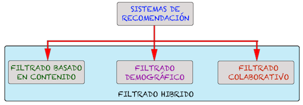
In this post we are going to focus on one part of collaborative filtering, more specifically memory-based collaborative filtering. Within recommender systems based on collaborative filtering, there are two classifications: memory-based and model-based.

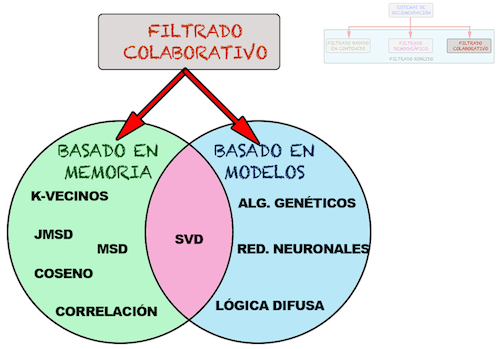
• Memory-based methods: they use similarity metrics to determine how alike two users are. To do so, they find the items that have been rated by both users and compare those ratings to calculate the similarity.
• Model-based methods: they use the ratings matrix to build a model through which to establish the set of users similar to the active user. Some examples of these models are Bayesian classifiers, neural networks, genetic algorithms, fuzzy systems and the matrix decomposition technique based on the SVD mathematical technique.

In this post we are going to explain the K-nearest neighbors technique for making recommendations, which falls within the memory-based methods. This technique is perhaps (not counting SVD) the best technique for making recommendations, since it is based on recommending to a user (from now on, the active user) the items (movies, books, trips, etc.) that users with tastes similar to the active user’s have liked, hence the name k-neighbors, where neighbors are users with tastes similar to the active user. For example, if user U1 liked the movies “The Godfather”, “Terminator” and “The Hangover”, and the active user (Ua) also liked “The Godfather” and “Terminator”, it is very likely that, since their tastes are very similar, the active user will also like “The Hangover”, so the recommender system should recommend this movie to the active user. This is a very basic example to understand the concept of the k-neighbors technique, which we will show in more detail later.

Let’s look at an example of a website dedicated to recommending movies and series (using the K-neighbors technique): FilmAffinity. This website has thousands of movies registered and must also have thousands of registered users to whom it has to make recommendations. To recommend to a user with this K-neighbors technique, the user must first “rate” a series of movies (on this site they do it with scores from 1 to 10) so that their tastes are known. In turn, the other thousands of users (among whom there is surely someone with tastes similar to the active user’s) must have rated a series of movies. This gives us what is called the “Ratings Matrix“, which represents the ratings users have given to movies. Needless to say, this ratings matrix is going to be very sparse; that is, users will rate a very small percentage of movies, since if there are thousands of movies in the website’s database, the average user (unless they are a film buff) will have rated about 100-200 movies. With this ratings matrix, we can calculate what is called the “Similarity between users“, which is simply a value (usually between 0 and 1) that tells us how similar we are to other users. We calculate this similarity between users with one of the similarity metrics that exist for recommender systems. The best-known metrics (and the ones we are going to explain here) are MSD (mean squared difference), the Pearson Correlation and the Cosine. There are other metrics that are much better than these, such as the JMSD metric and the Singularities metric, which we won’t explain because of their relative complexity, but we mention them and give you the links to their articles in case you want to check them out. Next we are going to show the three proposed similarity metrics, which basically calculate “the distances” between each pair of users:

1.-MSD (Minimun Square Difference):

Where #B_x,y is the number of movies that both users have rated (which must necessarily be greater than 0); r_x,i and r_y,i are the ratings given by users x and y respectively, and max and min are the maximum and minimum scores that users have given.

2.-Pearson Correlation:

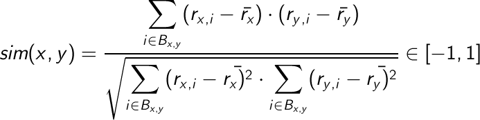
Where r_x with a “little hat” is the average rating of user x.

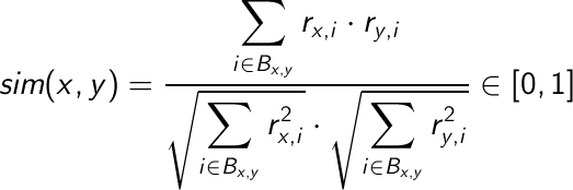
3.-Cosine: it measures the distance between two users based on the angle they form with each other.

And at this point, what does the K-neighbors technique consist of? Quite simple: this technique consists of following a series of steps to make recommendations, namely the following 4 steps (general scheme of collaborative filtering):

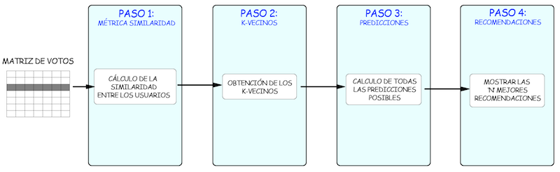
1. Calculating the similarity between users: First, you have to choose a metric (MSD, Cosine, …) to determine the similarity between a pair of users.
2. Calculating the K-neighbors: Using the selected similarity metric, you get the k users most similar to the active user. These users are called the k-neighbors of the active user.
3. Calculating the item predictions: From the k-neighbors of the active user, you determine the likely ratings the active user would give to the items they haven’t rated; that is, you predict how the user would rate those items.
4. Making the recommendations: After calculating the predictions, you choose the N most suitable items to recommend to the user, that is, the highest predictions, the newest, the most rated, etc. Optionally, you can include a threshold to prevent items with a prediction below it from being recommended.

At this point, we have seen the K-neighbors technique from a very theoretical point of view, so let’s go through an example of how to recommend given the following ratings matrix, in which users rate on a scale from 1 to 5 (instead of 1 to 10):

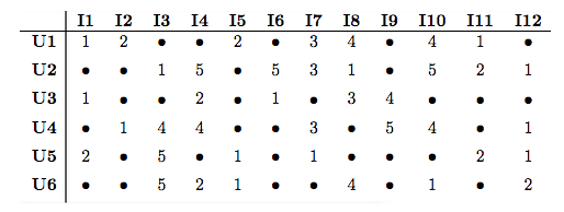
The positions with the symbol “•” mean that the user has not rated the corresponding item.

Once you have the ratings matrix, you have to calculate the similarities a user has with the rest of the users in the database. As an example, we are going to show how to calculate the similarity between users U1 and U2 using the MSD similarity metric:

We show the similarities between each pair of users in the following table. We calculated these similarities using the MSD metric, and you can do the calculations for each pair of users to check that you are calculating the similarity between each pair of users correctly:

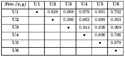
At this point we have to sort the similarities from highest to lowest for each user and take as many neighbors as we want, so that we can later predict the user’s ratings. In this case we are going to take two neighbors, so we can see that the two users most similar to user U1 are users U4 and U3, since they have the highest similarity. In the following table we show the two neighbors for each user:

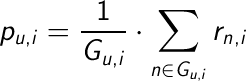
Once we have chosen the neighbors, all that’s left is to predict the ratings a user would give to the items they haven’t rated. This prediction can be made with the arithmetic mean of the neighbors’ ratings or with the weighted mean of the neighbors’ ratings, taking into account the similarity between them. The formulas for the weighted mean and the arithmetic mean are the following:

1.- Arithmetic mean:

2.- Weighted mean:

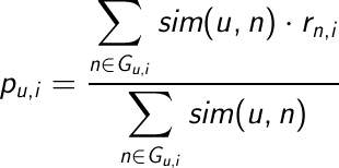
As an example, let’s calculate the prediction for item I1 that user U4 would make, given that their neighbors are users U1 and U5, with a similarity of 0.979 and 0.896 respectively:

1.- Arithmetic mean:

 

2.- Weighted mean:

 

To simplify the calculations, we show all the predictions for all the items for which predictions can be calculated, with the predictions for the items the user has not rated shown in blue:

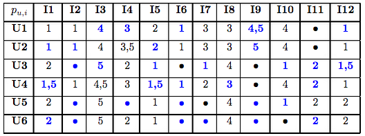
Once the predictions for the items the user hasn’t rated have been obtained, all that’s left is to make the recommendations, which is done by sorting the predictions from highest to lowest and recommending those with the highest predicted score. For example, for user U1 the first item to recommend would be item I9, since it has been predicted that the user will rate that item with a 4.5, then item I3 would be recommended, and so on. What is usually done in recommender systems is to recommend a fixed number of items; for example, 20 movies, 10 books, etc., which will correspond to the best predictions. To finish this example, let’s suppose that our recommender system is going to recommend only two items, so in the following table we show which items are candidates to be recommended to each user and which ones are actually recommended:

In short, this is the K-neighbors technique, and we have given a simple example of how to make recommendations. This example was taken from the master’s thesis of Ricardo Moya (co-creator of this website), from chapter 2, which covers the state of the art of recommender systems, and which you can see at the following link “SVD Applied to Recommender Systems Based on Collaborative Filtering (TFM) “ to expand your knowledge of these topics and of the SVD technique, which we will discuss later in other posts.

BIBLIOGRAPHY

Part of the information shown in this post was obtained from the classes of the course “Recommender Systems” taught in the Master’s in “Computer Science and Technology” at the Escuela Universitaria de Informática of the UPM by Professor and Doctor Antonio Hernando and also from the master’s thesis of EUI professor and researcher Fernando Ortega, both of them great experts in Recommender Systems who have published numerous JCR articles on the subject and who are the creators of the JMSD and Singularities metrics (together with Jesus Bobadilla and Jesus Bernal) mentioned in this post.