CPU vs GPU in Deep Learning: How Big Is the Difference in Training Time?

You can download the code for this post from GitHub by clicking HERE.

Using GPUs in Deep Learning (Neural Networks) to train models is becoming more and more common because of the significant reduction in training times. But can we actually quantify how big the difference in model training time is between a CPU and a GPU? If we search the internet, we will surely find conclusions such as using a GPU is between 8 and 12 times faster than using a CPU, and indeed, depending on the problem to solve and the hardware we use, that could be the range of improvement in times between a GPU and a CPU. In the example we are going to show below, we will see how training the model with the GPU is 9.6 times faster than with the CPU:

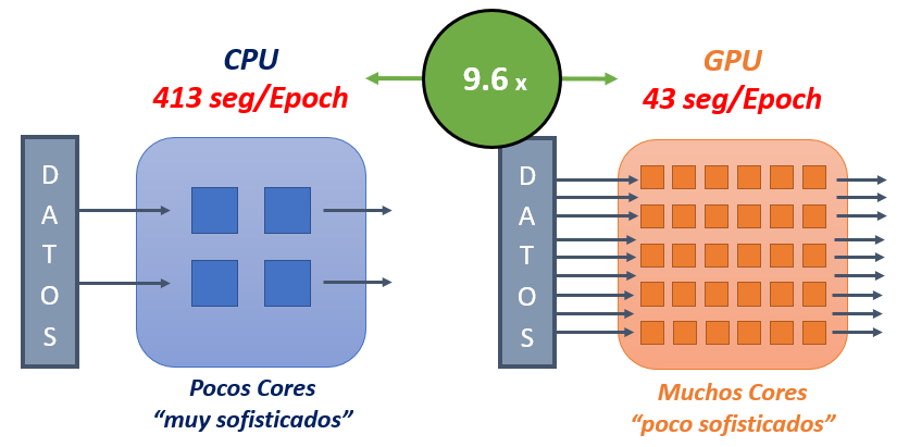
So, to demonstrate the improvement in training times for a Deep Learning model between a CPU and a GPU, we are going to solve an “Image Classification with Convolutional Neural Networks with TensorFlow” problem and see empirically the time differences between training it with a CPU and with a GPU.

Hardware used for the experiment

For the experiments we have a laptop with the following CPU and GPU:

• CPU: intel core i7 10750h / 2.6 ghz
• GPU: NVIDIA GeForce RTX 2060 8GB

Python virtual environment for the execution

We are going to create a new virtual environment with Anaconda with Python 3.7, where we will install version 2.7.0 of tensorflow-gpu. To create the new environment (which we will call “test_tiempos_gpu_cpu”) we open an Anaconda terminal and type:

>> conda create -n test_tiempos_gpu_cpu python=3.7

Once it is installed, we activate the environment as follows

>> conda activate test_tiempos_gpu_cpu

And we install version 2.7.0 of tensorflow with pip

>> pip install tensorflow-gpu==2.7.0

The GPU was previously correctly configured with the Drivers, CUDA 11.2 and cuDNN 8.1

Dataset

The Dataset with the images to classify was obtained from Kaggle: 8 kinds of image classification (Kaggle)

To run this project (either in the notebook or in the Script) you must download this Dataset and save it in the project’s “data” folder.

This Dataset contains 3 folders (pred, test and train) with 35,000 images classified into 8 different classes: seas, streets, buildings, glaciers, mountains, forests, cats, and dogs.

Execution script details

Printing the TensorFlow version, the CUDA and cuDNN versions and the available GPU

We get this information with the following code snippet:

import tensorflow.keras

from tensorflow.python.client import device_lib

print('#### INFORMACIÓN ####')
print('  Versión de TensorFlow: {}'.format(tensorflow.__version__))
print('  GPU: {}'.format([x.physical_device_desc for x in device_lib.list_local_devices() if x.device_type == 'GPU']))
print('  Versión Cuda  -> {}'.format(tensorflow.sysconfig.get_build_info()['cuda_version']))
print('  Versión Cudnn -> {}\n'.format(tensorflow.sysconfig.get_build_info()['cudnn_version']))

Getting as output

#### INFORMACIÓN ####
  Versión de TensorFlow: 2.7.0
  GPU: ['device: 0, name: NVIDIA GeForce RTX 2060, pci bus id: 0000:01:00.0, compute capability: 7.5']
  Versión Cuda  -> 64_112
  Versión Cudnn -> 64_8

Loading the training and test images

The test and train folders, which are the ones we are going to use, each contain another 8 folders, one for each category, and in each of those folders are the images classified by category. Here is the folder structure:

data
├── test
│   ├── buildings
│   ├── cat
│   ├── dog
│   ├── forest
│   ├── glacier
│   ├── mountain
│   ├── sea
│   └── street
└── train
    ├── buildings
    ├── cat
    ├── dog
    ├── forest
    ├── glacier
    ├── mountain
    ├── sea
    └── street

For this experiment, we are going to create two objects of the ImageDataGenerator class, which, given a folder (in our case the train and test folders), will generate as many images as we tell it to for training the model and for validating it (the set of test images).

We will “create” as many images as we tell the ImageDataGenerator class to, since it can generate new images from a given one by applying certain modifications such as rotations or zooms.

For this experiment we are going to create 2 sets of images:

• train_generator: from the train images folder, it will resize the images to 150×150 (PIXELES) and generate groups of 32 images (BATCH_SIZE), normalized and able to apply rotations (rotation_range) of 20 degrees and zoom of up to 20% (zoom_range), and also able to modify up to 20% of a photo’s pixels (shear_range).
• test_generator: from the test images folder, it will resize the images to 150×150 (PIXELES) and generate groups of 32 images (BATCH_SIZE), normalized. Since these images represent “reality”, we will not modify them.

from tensorflow.keras.preprocessing.image import ImageDataGenerator


# CONSTANTS:
PIXELES = 150                   # Height and width pixels of the image e.g.-> (150,150)
NUM_EPOCHS = 10                 # Number of epochs
BATCH_SIZE = 32                 # Number of images per batch
NUM_BATCHES_PER_EPOCH = 1000    # Number of batches to run in each EPOCH

# We define how to randomly modify the training images (pixels)
#   https://www.tensorflow.org/api_docs/python/tf/keras/preprocessing/image/ImageDataGenerator
#   rescale = normalize the pixels
#   shear_range = random modification range
#   zoom_range = random zoom range
#   ratation_range = maximum random rotation angle of the image
#   horizontal_flip = random flip of the images
train_datagen = ImageDataGenerator(rescale=1. / 255,
                                   shear_range=0.2,
                                   zoom_range=0.2,
                                   rotation_range=20,
                                   horizontal_flip=True)

# We define how to modify the test images (pixels)
#   rescale = normalize the pixels
test_datagen = ImageDataGenerator(rescale=1. / 255)

# We define what our training and test images look like
#   directory = path where the images are (one class per folder)
#   target_size = size of the images 150x150. They are resized to that size
#   batch_size = Number of images after which the network weights will be computed
#   class_mode = classification type: binary
train_generator = train_datagen.flow_from_directory(directory='./data/train',
                                                    target_size=(PIXELES, PIXELES),
                                                    batch_size=BATCH_SIZE,
                                                    class_mode='categorical')

test_generator = test_datagen.flow_from_directory(directory='./data/test',
                                                  target_size=(PIXELES, PIXELES),
                                                  batch_size=BATCH_SIZE,
                                                  class_mode='categorical')

num_classes = train_generator.num_classes
print("Nº de Imágenes para entrenamiento: {}".format(train_generator.n))
print("Nº de Imágenes para test: {}".format(test_generator.n))
print("Nº de Clases a Clasificar: {} Clases".format(num_classes))

Running this code snippet shows that we have 18687 images available for training and 4463 images for testing, across 8 different classes. From these images, we will generate as many images as we want by modifying them as mentioned above

Found 18687 images belonging to 8 classes.
Found 4463 images belonging to 8 classes.
Nº de Imágenes para entrenamiento: 18687
Nº de Imágenes para test: 4463
Nº de Clases a Clasificar: 8 Clases

Defining the Convolutional Neural Network (CNN) model

We define a neural network with the following architecture:

1. Input images: 150 pixels wide, 150 pixels high, 3 channels
2. Convolutional layer: 32 filters, kernel (3×3), RELU activation function
3. MaxPooling: Reduction of (2,2)
4. Convolutional layer: 64 filters, kernel (3×3), RELU activation function
5. MaxPooling: Reduction of (2,2)
6. Flatten layer: Input layer of the classifier. Feeds each pixel to a neuron
7. Hidden layer 1: 512 neurons, RELU activation function
8. Hidden layer 2: 64 neurons, RELU activation function
9. Output layer: 8 neurons (8 classes), SOFTMAX activation function

The model will have 42 million parameters (exactly 42,520,584 parameters)

To optimize the parameters of the network we will use:

• Loss function: categorical_crossentropy
• Optimizer: ADAM
• Metrics to monitor: Accuracy

from tensorflow.keras.models import Sequential
from tensorflow.keras.layers import Conv2D
from tensorflow.keras.layers import MaxPooling2D
from tensorflow.keras.layers import Flatten
from tensorflow.keras.layers import Dense
from tensorflow.keras.layers import Dropout


# We define the model
model = Sequential()
model.add(Conv2D(filters=32,
                 kernel_size=(3, 3),
                 input_shape=(PIXELES, PIXELES, 3),
                 activation='relu'))
model.add(MaxPooling2D(pool_size=(2, 2)))
model.add(Conv2D(filters=64,
                 kernel_size=(3, 3),
                 activation='relu'))
model.add(MaxPooling2D(pool_size=(2, 2)))
model.add(Flatten())
model.add(Dense(512, activation='relu'))
model.add(Dropout(0.2))
model.add(Dense(64, activation='relu'))
model.add(Dropout(0.2))
model.add(Dense(num_classes, activation='softmax'))

# We print the architecture of the defined network
print(model.summary())

# We compile the model
model.compile(loss='categorical_crossentropy', optimizer='adam', metrics=['categorical_accuracy'])

Calling the “summary()” function prints the layers of the neural network and the number of parameters (weights) of each layer:

_____________________________________________________________________________
| Layer (type)                      |   Output Shape          |   Param     |
|===================================|=========================|=============|
| conv2d (Conv2D)                   |   (None, 148, 148, 32)  |   896       |
| max_pooling2d (MaxPooling2D)      |   (None, 74, 74, 32)    |   0         |                                                          
| conv2d_1 (Conv2D)                 |   (None, 72, 72, 64)    |   18496     |
| max_pooling2d_1 (MaxPooling2D)    |   (None, 36, 36, 64)    |   0         |
| flatten (Flatten)                 |   (None, 82944)         |   0         |
| dense (Dense)                     |   (None, 512)           |   42467840  |
| dropout (Dropout)                 |   (None, 512)           |   0         |
| dense_1 (Dense)                   |   (None, 64)            |   32832     |
| dropout_1 (Dropout)               |   (None, 64)            |   0         |
| dense_2 (Dense)                   |   (None, 8)             |   520       |
|============================================================================
Total params: 42,520,584
Trainable params: 42,520,584
Non-trainable params: 0
_____________________________________________________________________________

Training the network with the GPU

For training the model on both the GPU and the CPU we will use:

• epochs: 5 epochs
• steps_per_epoch: Each epoch will have 1000 batches of 32 images
• training images: images loaded in the train_generator variable of the ImageDataGenerator class
• test images: after each epoch, 320 images will be validated (10 batches – validation_steps – of 32 images) loaded in the test_generator variable of the ImageDataGenerator class
• workers: number of threads (12) for parallel processing on the CPU. When training with the GPU, the CPU is in charge of passing the batches with the training images to the GPU.

# CONSTANTS:
NUM_EPOCHS = 5                  # Number of epochs
NUM_BATCHES_PER_EPOCH = 1000    # Number of batches to run in each EPOCH

# Run with GPU
try:
    with tensorflow.device('/gpu:0'):
        print("### EJECUCIÓN CON GPU ###")
        model.fit(train_generator,
                  epochs=NUM_EPOCHS,
                  steps_per_epoch=NUM_BATCHES_PER_EPOCH,
                  validation_data=test_generator,
                  validation_steps=10,
                  workers=12,
                  verbose=1)
except Exception as e:
    print('WARNING: No es posible ejecutar con GPU: {}'.format(e))

After training the model with the GPU, we can see in the output that it takes between 38 and 45 seconds per epoch. Remember that in each epoch there are 1000 batches of 32 images; that is, during training the network is fed 32 images (1000 times), and after classifying the 32 images, it computes the classification error and adjusts the network’s 42 million parameters based on that error. So in each epoch the parameters (or weights) of the neural network are adjusted 1000 times.

### EJECUCIÓN CON GPU ###
Epoch 1/5
1000/1000 [==============================] - 38s 35ms/step - loss: 1.0006 - categorical_accuracy: 0.6425 - val_loss: 0.8249 - val_categorical_accuracy: 0.6938
Epoch 2/5
1000/1000 [==============================] - 42s 42ms/step - loss: 0.6830 - categorical_accuracy: 0.7616 - val_loss: 0.8725 - val_categorical_accuracy: 0.7000
Epoch 3/5
1000/1000 [==============================] - 45s 44ms/step - loss: 0.6058 - categorical_accuracy: 0.7910 - val_loss: 0.8989 - val_categorical_accuracy: 0.6938
Epoch 4/5
1000/1000 [==============================] - 44s 43ms/step - loss: 0.5522 - categorical_accuracy: 0.8094 - val_loss: 0.8550 - val_categorical_accuracy: 0.7094
Epoch 5/5
1000/1000 [==============================] - 45s 45ms/step - loss: 0.5181 - categorical_accuracy: 0.8197 - val_loss: 0.7174 - val_categorical_accuracy: 0.7594

Training the network with the CPU

The code for training the model with the CPU is:

# Run with CPU
try:
    with tensorflow.device('/cpu:0'):
        print("### EJECUCIÓN CON CPU ###")
        model.fit(train_generator,
                  epochs=NUM_EPOCHS,
                  steps_per_epoch=NUM_BATCHES_PER_EPOCH,
                  validation_data=test_generator,
                  validation_steps=10,
                  workers=12,
                  verbose=1)
except Exception as e:
    print('WARNING: No es posible ejecutar con CPU: {}'.format(e))

When training the model with the CPU, we can see that it takes between 408 and 424 seconds per epoch (about 7 minutes).

### EJECUCIÓN CON CPU ###
Epoch 1/5
1000/1000 [==============================] - 424s 423ms/step - loss: 0.4764 - categorical_accuracy: 0.8343 - val_loss: 0.6885 - val_categorical_accuracy: 0.7406
Epoch 2/5
1000/1000 [==============================] - 413s 413ms/step - loss: 0.4569 - categorical_accuracy: 0.8416 - val_loss: 0.9499 - val_categorical_accuracy: 0.6969
Epoch 3/5
1000/1000 [==============================] - 413s 412ms/step - loss: 0.4339 - categorical_accuracy: 0.8497 - val_loss: 0.6461 - val_categorical_accuracy: 0.7688
Epoch 4/5
1000/1000 [==============================] - 408s 408ms/step - loss: 0.4117 - categorical_accuracy: 0.8571 - val_loss: 0.6222 - val_categorical_accuracy: 0.7812
Epoch 5/5
1000/1000 [==============================] - 408s 407ms/step - loss: 0.3941 - categorical_accuracy: 0.8617 - val_loss: 0.7112 - val_categorical_accuracy: 0.7906

Conclusions

In this experiment we have shown how, by using a GPU instead of a CPU to train a Deep Learning model, the training time is almost 10 times shorter (9.6 times), with a GPU training time of 43 seconds for 1 epoch of 1000 batches of 32 images. For training with the CPU this time (on average) was 413 seconds.

FULL CODE AND EXECUTION

# -*- coding: utf-8 -*-
__author__ = 'RicardoMoya'

import tensorflow.keras

from tensorflow.keras.models import Sequential
from tensorflow.keras.layers import Conv2D
from tensorflow.keras.layers import MaxPooling2D
from tensorflow.keras.layers import Flatten
from tensorflow.keras.layers import Dense
from tensorflow.keras.layers import Dropout
from tensorflow.keras.preprocessing.image import ImageDataGenerator
from tensorflow.python.client import device_lib

print('#### INFORMACIÓN ####')
print('  Versión de TensorFlow: {}'.format(tensorflow.__version__))
print('  GPU: {}'.format([x.physical_device_desc for x in device_lib.list_local_devices() if x.device_type == 'GPU']))
print('  Versión Cuda  -> {}'.format(tensorflow.sysconfig.get_build_info()['cuda_version']))
print('  Versión Cudnn -> {}\n'.format(tensorflow.sysconfig.get_build_info()['cudnn_version']))


# CONSTANTS:
PIXELES = 150                   # Height and width pixels of the image e.g.-> (150,150)
NUM_EPOCHS = 5                  # Number of epochs
BATCH_SIZE = 32                 # Number of images per batch
NUM_BATCHES_PER_EPOCH = 1000    # Number of batches to run in each EPOCH

# We define how to randomly modify the training images (pixels)
#   https://www.tensorflow.org/api_docs/python/tf/keras/preprocessing/image/ImageDataGenerator
#   rescale = normalize the pixels
#   shear_range = random modification range
#   zoom_range = random zoom range
#   ratation_range = maximum random rotation angle of the image
#   horizontal_flip = random flip of the images
train_datagen = ImageDataGenerator(rescale=1. / 255,
                                   shear_range=0.2,
                                   zoom_range=0.2,
                                   rotation_range=20,
                                   horizontal_flip=True)

# We define how to modify the test images (pixels)
#   rescale = normalize the pixels
test_datagen = ImageDataGenerator(rescale=1. / 255)

# We define what our training and test images look like
#   directory = path where the images are (one class per folder)
#   target_size = size of the images 150x150. They are resized to that size
#   batch_size = Number of images after which the network weights will be computed
#   class_mode = classification type: multiple
train_generator = train_datagen.flow_from_directory(directory='./data/train',
                                                    target_size=(PIXELES, PIXELES),
                                                    batch_size=BATCH_SIZE,
                                                    class_mode='categorical')

test_generator = test_datagen.flow_from_directory(directory='./data/test',
                                                  target_size=(PIXELES, PIXELES),
                                                  batch_size=BATCH_SIZE,
                                                  class_mode='categorical')

num_classes = train_generator.num_classes
print("Nº de Imagenes para entrenamiento: {}".format(train_generator.n))
print("Nº de Imagenes para test: {}".format(test_generator.n))
print("Nº de Clases a Clasificar: {} Clases".format(num_classes))

# We define the model
#   Input images: 150 pixels wide, 150 pixels high, 3 channels
#   Convolutional layer: 32 filters, kernel (3x3), RELU activation function
#   MaxPooling: Reduction of (2,2)
#   Convolutional layer: 64 filters, kernel (3x3), RELU activation function
#   MaxPooling: Reduction of (2,2)
#   Flatten layer: Input layer of the classifier. Feeds each pixel to a neuron
#   Hidden layer 1: 512 neurons, RELU activation function
#   Hidden layer 2: 64 neurons, RELU activation function
#   Output layer: 8 neurons (8 classes), SOFTMAX activation function
model = Sequential()
model.add(Conv2D(filters=32,
                 kernel_size=(3, 3),
                 input_shape=(PIXELES, PIXELES, 3),
                 activation='relu'))
model.add(MaxPooling2D(pool_size=(2, 2)))
model.add(Conv2D(filters=64,
                 kernel_size=(3, 3),
                 activation='relu'))
model.add(MaxPooling2D(pool_size=(2, 2)))
model.add(Flatten())
model.add(Dense(512, activation='relu'))
model.add(Dropout(0.2))
model.add(Dense(256, activation='relu'))
model.add(Dropout(0.2))
model.add(Dense(num_classes, activation='softmax'))

# We print the architecture of the defined network
print(model.summary())

# We compile the model
#   Loss function: categorical_crossentropy
#   Optimizer: ADAM
#   Metrics to monitor: Accuracy
model.compile(loss='categorical_crossentropy', optimizer='adam', metrics=['categorical_accuracy'])

# Model fitting
#   epochs = number of epochs
#   steps_per_epoch = Number of batches per epoch
#   validation_data = Test (validation) images
#   validation_steps = Number of batches (1 batch = BACH_SIZE images) of images to validate per epoch
#   workers = number of threads for parallel processing on the CPU

# Run with GPU
try:
    with tensorflow.device('/gpu:0'):
        print("### EJECUCIÓN CON GPU ###")
        model.fit(train_generator,
                  epochs=NUM_EPOCHS,
                  steps_per_epoch=NUM_BATCHES_PER_EPOCH,
                  validation_data=test_generator,
                  validation_steps=10,
                  workers=12,
                  verbose=1)
except Exception as e:
    print('WARNING: No es posible ejecutar con GPU: {}'.format(e))

# Run with CPU
try:
    with tensorflow.device('/cpu:0'):
        print("### EJECUCIÓN CON CPU ###")
        model.fit(train_generator,
                  epochs=NUM_EPOCHS,
                  steps_per_epoch=NUM_BATCHES_PER_EPOCH,
                  validation_data=test_generator,
                  validation_steps=10,
                  workers=12,
                  verbose=1)
except Exception as e:
    print('WARNING: No es posible ejecutar con CPU: {}'.format(e))

#### INFORMACIÓN ####
  Versión de TensorFlow: 2.7.0
  GPU: ['device: 0, name: NVIDIA GeForce RTX 2060, pci bus id: 0000:01:00.0, compute capability: 7.5']
  Versión Cuda  -> 64_112
  Versión Cudnn -> 64_8


Found 18687 images belonging to 8 classes.
Found 4463 images belonging to 8 classes.
Nº de Imagenes para entrenamiento: 18687
Nº de Imagenes para test: 4463
Nº de Clases a Clasificar: 8 Clases


Model: "sequential"
_____________________________________________________________________________
| Layer (type)                      |   Output Shape          |   Param #   |
|===================================|=========================|=============|
| conv2d (Conv2D)                   |   (None, 148, 148, 32)  |   896       |
| max_pooling2d (MaxPooling2D)      |   (None, 74, 74, 32)    |   0         |                                                          
| conv2d_1 (Conv2D)                 |   (None, 72, 72, 64)    |   18496     |
| max_pooling2d_1 (MaxPooling2D)    |   (None, 36, 36, 64)    |   0         |
| flatten (Flatten)                 |   (None, 82944)         |   0         |
| dense (Dense)                     |   (None, 512)           |   42467840  |
| dropout (Dropout)                 |   (None, 512)           |   0         |
| dense_1 (Dense)                   |   (None, 64)            |   32832     |
| dropout_1 (Dropout)               |   (None, 64)            |   0         |
| dense_2 (Dense)                   |   (None, 8)             |   520       |
|============================================================================
Total params: 42,520,584
Trainable params: 42,520,584
Non-trainable params: 0
_____________________________________________________________________________
None
### EJECUCIÓN CON GPU ###
Epoch 1/5
1000/1000 [==============================] - 38s 35ms/step - loss: 1.0006 - categorical_accuracy: 0.6425 - val_loss: 0.8249 - val_categorical_accuracy: 0.6938
Epoch 2/5
1000/1000 [==============================] - 42s 42ms/step - loss: 0.6830 - categorical_accuracy: 0.7616 - val_loss: 0.8725 - val_categorical_accuracy: 0.7000
Epoch 3/5
1000/1000 [==============================] - 45s 44ms/step - loss: 0.6058 - categorical_accuracy: 0.7910 - val_loss: 0.8989 - val_categorical_accuracy: 0.6938
Epoch 4/5
1000/1000 [==============================] - 44s 43ms/step - loss: 0.5522 - categorical_accuracy: 0.8094 - val_loss: 0.8550 - val_categorical_accuracy: 0.7094
Epoch 5/5
1000/1000 [==============================] - 45s 45ms/step - loss: 0.5181 - categorical_accuracy: 0.8197 - val_loss: 0.7174 - val_categorical_accuracy: 0.7594
### EJECUCIÓN CON CPU ###
Epoch 1/5
1000/1000 [==============================] - 424s 423ms/step - loss: 0.4764 - categorical_accuracy: 0.8343 - val_loss: 0.6885 - val_categorical_accuracy: 0.7406
Epoch 2/5
1000/1000 [==============================] - 413s 413ms/step - loss: 0.4569 - categorical_accuracy: 0.8416 - val_loss: 0.9499 - val_categorical_accuracy: 0.6969
Epoch 3/5
1000/1000 [==============================] - 413s 412ms/step - loss: 0.4339 - categorical_accuracy: 0.8497 - val_loss: 0.6461 - val_categorical_accuracy: 0.7688
Epoch 4/5
1000/1000 [==============================] - 408s 408ms/step - loss: 0.4117 - categorical_accuracy: 0.8571 - val_loss: 0.6222 - val_categorical_accuracy: 0.7812
Epoch 5/5
1000/1000 [==============================] - 408s 407ms/step - loss: 0.3941 - categorical_accuracy: 0.8617 - val_loss: 0.7112 - val_categorical_accuracy: 0.7906