
Expectation-Maximization in Python and Scikit-learn, with Examples
Expectation-maximization is a statistical clustering method similar to K-means, but with a probabilistic approach. Learn how it works with Python examples.
Tool
- You can download the project for this post by clicking HERE.
- This post is part of the book "Machine Learning (in Python), with Examples"
Expectation-maximization (EM) is a statistical Clustering method similar to K-means, but with a probabilistic approach. This method assumes that all the objects (in the data set) have been generated from ‘k’ probability distributions whose parameters we don’t know a priori.
To understand what we want to solve with EM, let’s suppose the following case, in which we know that two groups of objects (Clusters) are generated according to two normal (Gaussian) distributions p(x|μ,σ) defined by their mean (μ) and their standard deviation (σ):
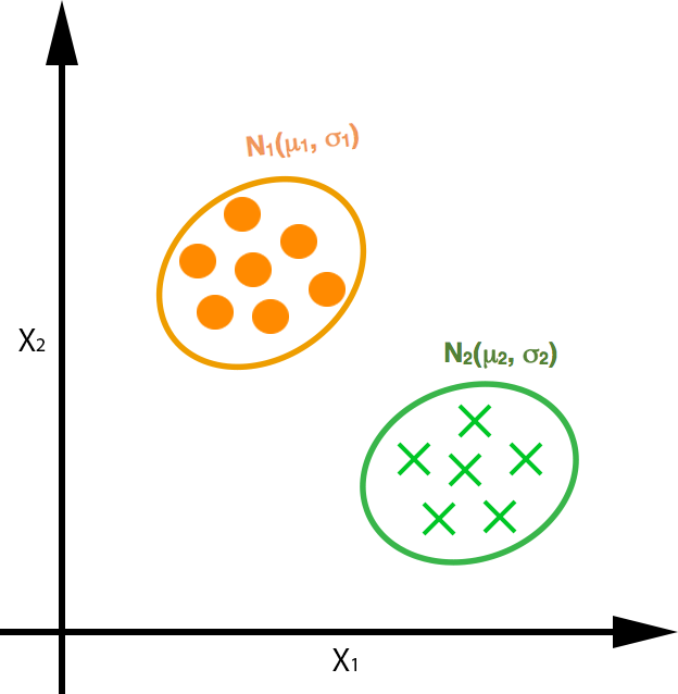
In this example we know the parameters of the normal distributions (the mean and standard deviation), and therefore, given any point, we can tell which Cluster it belongs to, or which probability distribution it belongs to (or is more likely to belong to).
Now let’s flip the problem around: we have a set of objects and we don’t know the parameters of the probability distributions that generate them (for a normal distribution, its mean and standard deviation). In other words, the data set doesn’t give us enough information to know how the assumed probabilistic models were created. This lack of information (or missing information) in the training data is called “missing data” or “latent variables”.
The goal of EM is therefore to find, from the training data (data set), the parameters of the probability distributions that we assume generated this data; or, put a bit more formally, to find maximum likelihood estimates of the parameters of statistical models that depend on latent variables.
Although EM can be applied to any probability distribution (it doesn’t have to be only normal distributions, since we don’t know the nature of the data we have), next we’re going to explain in detail the calculations and steps needed to compute the parameters of ‘k’ normal distributions, assuming the objects in our data set were generated according to ‘k’ normal distributions p(x|μ,σ); that way, we can group this data into ‘k’ Clusters.
As with K-means, we must define beforehand how many Clusters we’ll use to group the objects. Let’s suppose we choose 3 Clusters (K=3). Given an object from our data set, we assume it follows one of the three normal distributions; therefore, it will have a certain probability ‘π’ of belonging to each of the Clusters. A priori we say that it has a 33.3% chance of belonging to Cluster 1, a 33.3% chance of belonging to Cluster 2 and a 33.4% chance of belonging to Cluster 3. Once we know more about the objects in each Cluster, this probability per Cluster will change; for example, if we have 100 objects, of which 50 are in Cluster 1, 35 are in Cluster 2 and 15 are in Cluster 3, we say that given a point, it has a 50% chance of belonging to Cluster 1, a 35% chance of belonging to Cluster 2 and a 15% chance of belonging to Cluster 3.
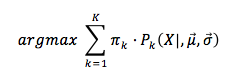
On the other hand, for each of the probability distributions we have to calculate its parameters; and in this case, assuming normal distributions, we must calculate the mean and standard deviation of each one based on the objects in the data set. As we adjust these values while the EM algorithm runs, each object in the data set will have a certain probability of belonging to each of the Clusters; therefore (and similarly to K-means with distances), each object will belong to the Cluster with the highest probability (the product πi · pi(x|μ,σ)).
Below is EM for normal (Gaussian) distributions shown in “Plate Notation” :
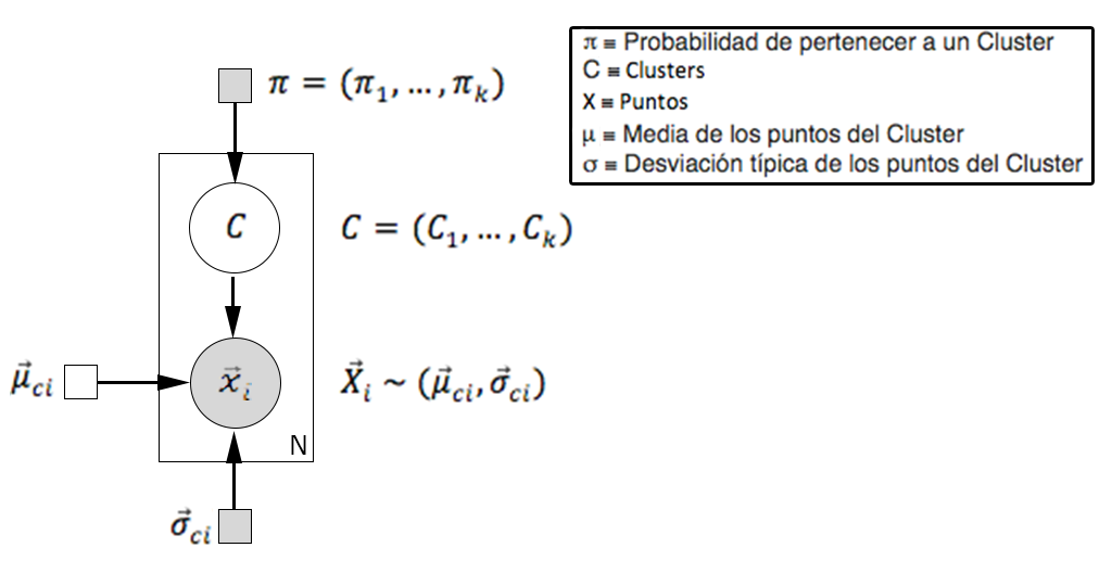
In the image above we define the circles as probability distributions and the squares as scalars or vectors, where gray backgrounds are known values or probability distributions and white backgrounds are unknown ones, which therefore have to be calculated. What the image represents is that we have ‘N’ objects, where each one of them ‘xi’ is in a probability distribution with an unknown mean ‘μi’ (which therefore has to be calculated) and a known standard deviation ‘σi’ . Each object can belong with a probability ‘πi’ to each of the ‘k’ Clusters ‘C’, finally assigning a specific object of the data set to the Cluster whose probability, defined as the product of ‘πi’ and pi(x|μi,σi), is the highest of all.
The problem to solve is therefore calculating the probability that an object belongs to each of the Clusters. For that we have the following:

What we want to know is the probability that an object belongs to each of the Clusters:

On the other hand, P(C│π) is a constant value (P(c=1│π1 ), P(c=2│π2 ), …, P(c=k│π_k )), which helps us when calculating the probabilities, leaving it as follows:

Applying the density function of a normal distribution, the sum of all the probabilities that a point belongs to the Clusters is:
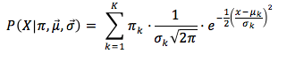
We can simplify this probability since 1/√2π is a constant, leaving:
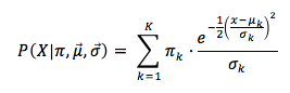
We can do this last step because what we care about is assigning the object to the Cluster with the highest probability; that is:
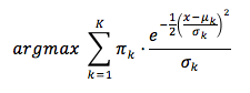
Once we’ve defined how to calculate the probability that an object belongs to a Cluster, let’s explain how EM works. As you’ll see, it behaves very much like K-means, with two steps: the expectation step and the maximization step, which are similar to the assignment and update steps of K-means, respectively.
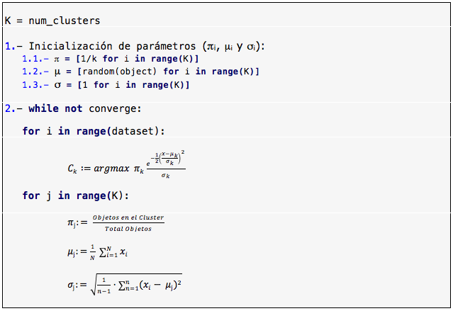
EM starts by initializing the parameters of the probability distributions and the probabilities of belonging to the Clusters. We can do this in many ways, for example by initializing the probability of belonging to a Cluster ‘π’ as 1/k, and for the normal distributions initializing the standard deviation to ‘1’ and the mean with the value of a point from the data set. Once the parameters are initialized, the algorithm keeps alternating the following two steps (expectation and maximization) iteratively until the means of the normal distributions converge:
- Expectation: With the known parameters of the normal distributions and the probability ‘π’ of belonging to a Cluster, assign each object to the Cluster with the highest membership probability:
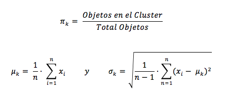
- Maximization: Using the objects assigned to each Cluster, calculate the value of the parameters (πk, μk and σk):
Now that we’ve defined how the algorithm works step by step, here it is in pseudocode:
In the next two sections, Implementation of Expectation-maximization and Expectation-maximization (Gaussian mixture models) with scikit-learn, we’ll show an implementation of EM assuming the data is generated from normal distributions, and the use of the scikit-learn library to solve a Clustering problem with the Gaussian mixture models algorithm, respectively. The code can be found in the following repository:
View on GitHubRicardoMoya/ExpectationMaximization_Python
The code in this repository uses the numpy, matplotlib, scipy and scikit-learn libraries. To download and install these libraries (or update them to the latest version with the -U option) with the pip package manager, run the following commands:
pip install -U numpy
pip install -U matplotlib
pip install -U scipy
pip install -U scikit-learn
Implementation of Expectation-maximization
In this section we’ll show the implementation of EM (from a didactic point of view) in which the objects are represented by a point in two dimensions {x,y}. The implementation in this example allows the objects to have more dimensions, but to keep the didactic perspective we show them in two dimensions so that we can visualize the results on a plane and thus understand how this method works.
To implement EM, we’ll have objects represented as 2D points, so we’ll implement a Point class (Point.py) to represent the objects. We’ll also implement a Cluster class (Cluster.py) to represent the Clusters, made up of a set of objects of the Point class. Finally, we’ll have a script (EM.py) with EM implemented for normal distributions, with its two steps, expectation and maximization, for ‘k’ Clusters. Below is a high-level class diagram of the proposed EM implementation:
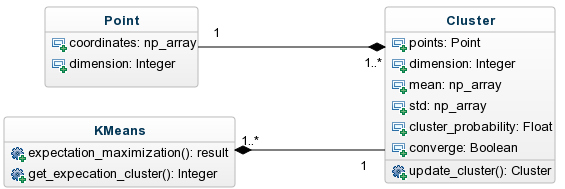
The data sets we’ll use in this example (located in the dataSet folder) are text files where each line holds the coordinates of a point {x,y} separated by the “::” separator. Here is an example of these files:
1.857611652::2.114033851
2.34822574::1.58264984
1.998326848::4.118143019
1.714362835::2.468639613
1.656134484::1.909955747
This means the first point is located at coordinates {1.85,2.11} and the second point at coordinates {2.34,1.58}.
For the examples we have 4 data sets with the following characteristics:
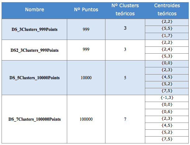
Now that we’ve seen the class diagram and the structure of the data sets, let’s show the implementation of the Point class (Point.py). This class receives a “numpy array” with the point’s coordinates in the constructor, and has as attributes those coordinates and their dimension, which for our example will be 2:
class Point:

    def __init__(self, coordinates):
        self.coordinates = coordinates
        self.dimension = len(coordinates)

    def __repr__(self):
        return 'Coordinates: ' + str(self.coordinates) + \
               '\n\t -> Dimension: ' + str(self.dimension)
On the other hand we have the Cluster class (Cluster.py), whose constructor receives a list of points that make up the Cluster and the total number of points. This class has as attributes the list of points in the Cluster (points), the dimension of the points (dimension), the mean of the points in the Cluster (mean), the standard deviation of the points in the Cluster (std), the probability ‘π’ of belonging to the Cluster (cluster_probability) and an attribute (converge) that tells us whether the mean is equal (and therefore converges) to the one calculated in the maximization step of the previous iteration. Here is the constructor of this class:
import numpy as np

class Cluster:

    def __init__(self, points, total_points):
        if len(points) == 0:
            raise Exception("Cluster cannot have 0 Points")
        else:
            self.points = points
            self.dimension = points[0].dimension

        # Check that all elements of the cluster have the same dimension
        for p in points:
            if p.dimension != self.dimension:
                raise Exception(
                    "Point %s has dimension %d different with %d from the rest "
                    "of points") % (p, len(p), self.dimension)

        # Calculate mean, std and probability
        points_coordinates = [p.coordinates for p in self.points]
        self.mean = np.mean(points_coordinates, axis=0)
        self.std = np.array([1.0, 1.0])
        self.cluster_probability = len(self.points) / float(total_points)
        self.converge = False
We also implement the update_cluster(points) method, which is in charge of updating the parameters of the probabilistic model that defines the Cluster, calculating the mean and standard deviation of the normal distribution and the probability ‘π’ of belonging to the Cluster; in short, this method performs the maximization step. This method also checks whether the means of the distribution converge from one iteration to the next. In summary, with this method we update the parameters of the probabilistic model that defines the Cluster.
def update_cluster(self, points, total_points):

    old_mean = self.mean
    self.points = points
    points_coordinates = [p.coordinates for p in self.points]
    self.mean = np.mean(points_coordinates, axis=0)
    self.std = np.std(points_coordinates, axis=0, ddof=1)
    self.cluster_probability = len(points) / float(total_points)
    self.converge = np.array_equal(old_mean, self.mean)
Now that we’ve explained the Point and Cluster classes we need to structure the information, let’s explain the EM implementation itself. This implementation is in the EM.py script shown below, and afterwards we’ll explain each relevant piece of code:
# -*- coding: utf-8 -*-
__author__ = 'RicardoMoya'

import random
import math
import numpy as np
import matplotlib.pyplot as plt
from matplotlib.patches import Ellipse
from Point import Point
from Cluster import Cluster

DATASET1 = "./dataSet/DS_3Clusters_999Points.txt"
DATASET2 = "./dataSet/DS2_3Clusters_999Points.txt"
DATASET3 = "./dataSet/DS_5Clusters_10000Points.txt"
DATASET4 = "./dataSet/DS_7Clusters_100000Points.txt"
NUM_CLUSTERS = 3
ITERATIONS = 1000
COLORS = ['red', 'blue', 'green', 'yellow', 'gray', 'pink', 'violet', 'brown',
          'cyan', 'magenta']


def dataset_to_list_points(dir_dataset):
    """
    Read a txt file with a set of points and return a list of objects Point
    :param dir_dataset: path file
    """
    points = list()
    with open(dir_dataset, 'rt') as reader:
        for point in reader:
            points.append(Point(np.asarray(map(float, point.split("::")))))
    return points


def get_probability_cluster(point, cluster):
    """
    Calculate the probability that the point belongs to the Cluster
    :param point:
    :param cluster:
    :return: probability =
    prob * SUM(e ^ (-1/2 * ((x(i) - mean)^2 / std(i)^2 )) / std(i))
    """
    mean = cluster.mean
    std = cluster.std
    prob = 1.0
    for i in range(point.dimension):
        prob *= (math.exp(-0.5 * (
            math.pow((point.coordinates[i] - mean[i]), 2) /
            math.pow(std[i], 2))) / std[i])

    return cluster.cluster_probability * prob


def get_expecation_cluster(clusters, point):
    """
    Returns the Cluster that has the highest probability of belonging to it
    :param clusters:
    :param point:
    :return: argmax (probability clusters)
    """
    expectation = np.zeros(len(clusters))
    for i, c in enumerate(clusters):
        expectation[i] = get_probability_cluster(point, c)

    return np.argmax(expectation)


def print_clusters_status(it_counter, clusters):
    print '\nITERATION %d' % it_counter
    for i, c in enumerate(clusters):
        print '\tCluster %d: Probability = %s; Mean = %s; Std = %s;' % (
            i + 1, str(c.cluster_probability), str(c.mean), str(c.std))


def print_results(clusters):
    print '\n\nFINAL RESULT:'
    for i, c in enumerate(clusters):
        print '\tCluster %d' % (i + 1)
        print '\t\tNumber Points in Cluster: %d' % len(c.points)
        print '\t\tProbability: %s' % str(c.cluster_probability)
        print '\t\tMean: %s' % str(c.mean)
        print '\t\tStandard Desviation: %s' % str(c.std)


def plot_ellipse(center, points, alpha, color):
    """
    Plot the Ellipse that defines the area of Cluster
    :param center:
    :param points: points of cluster
    :param alpha:
    :param color:
    :return: Ellipse
    """

    # Matrix Covariance
    cov = np.cov(points, rowvar=False)

    # eigenvalues and eigenvector of matrix covariance
    eigenvalues, eigenvector = np.linalg.eigh(cov)
    order = eigenvalues.argsort()[::-1]
    eigenvector = eigenvector[:, order]

    # Calculate Angle of ellipse
    angle = np.degrees(np.arctan2(*eigenvector[:, 0][::-1]))

    # Calculate with, height
    width, height = 4 * np.sqrt(eigenvalues[order])

    # Ellipse Object
    ellipse = Ellipse(xy=center, width=width, height=height, angle=angle,
                      alpha=alpha, color=color)

    ax = plt.gca()
    ax.add_artist(ellipse)

    return ellipse


def plot_results(clusters):
    plt.plot()
    for i, c in enumerate(clusters):
        # plot points
        x, y = zip(*[p.coordinates for p in c.points])
        plt.plot(x, y, linestyle='None', color=COLORS[i], marker='.')
        # plot centroids
        plt.plot(c.mean[0], c.mean[1], 'o', color=COLORS[i],
                 markeredgecolor='k', markersize=10)
        # plot area
        plot_ellipse(c.mean, [p.coordinates for p in c.points], 0.2, COLORS[i])

    plt.show()


def expectation_maximization(dataset, num_clusters, iterations):
    # Read data set
    points = dataset_to_list_points(dataset)

    # Select N points random to initiacize the N Clusters
    initial = random.sample(points, num_clusters)

    # Create N initial Clusters
    clusters = [Cluster([p], len(initial)) for p in initial]

    # Inicialize list of lists to save the new points of cluster
    new_points_cluster = [[] for i in range(num_clusters)]

    converge = False
    it_counter = 0
    while (not converge) and (it_counter < iterations):
        # Expectation Step
        for p in points:
            i_cluster = get_expecation_cluster(clusters, p)
            new_points_cluster[i_cluster].append(p)

        # Maximization Step
        for i, c in enumerate(clusters):
            c.update_cluster(new_points_cluster[i], len(points))

        # Check that converge all Clusters
        converge = [c.converge for c in clusters].count(False) == 0

        # Increment counter and delete lists of clusters points
        it_counter += 1
        new_points_cluster = [[] for i in range(num_clusters)]

        # Print clusters status
        print_clusters_status(it_counter, clusters)

    # Print final result
    print_results(clusters)

    # Plot Final results
    plot_results(clusters)


if __name__ == '__main__':
    expectation_maximization(DATASET1, NUM_CLUSTERS, ITERATIONS)
The first thing that happens when the script runs is a call to the expectation_maximization() method, which receives as parameters the data set containing the set of points, the number of Clusters we want to obtain, and the maximum number of iterations to run in case the means of the probability distributions never converge. We define these parameters as constants in the script since we have 4 data sets available.
if __name__ == '__main__':
    expectation_maximization(DATASET1, NUM_CLUSTERS, ITERATIONS)
The expectation_maximization() method implements EM as indicated in the pseudocode shown earlier. First we read the data set from a file with the dataset_to_list_points(file) method and initialize the ‘N’ distributions that define the Clusters (num_clusteres), with the mean obtained by randomly selecting ‘N’ points from the data set. Then we run the expectation and maximization steps until they converge or until we reach the maximum number of iterations (iterations). We do this inside the “While” loop. In each iteration we assign each point of the data set to the probability distribution with the highest membership probability (the product πi • pi(x|μi,σi)) with the get_expectation_cluster() method, which returns the index of the distribution (or Cluster), and once assigned we recalculate the parameters of the probability distributions. Then we check for convergence to see whether we keep iterating or not. In the implementation we also see the print_clusters_status(), print_results() and plot_results() methods, which are helper methods we use to show the parameters of the probability distributions that define the Clusters in each iteration, and to display and plot (with the matplotlib library) the final result:
def expectation_maximization(dataset, num_clusters, iterations):

    points = dataset_to_list_points(dataset)

    # INITIALIZATION: Random selection of N points to initialize the mean of
    # the normal distributions that define a Cluster
    initial = random.sample(points, num_clusters)

    # Create N initial Clusters
    clusters = [Cluster([p], len(initial)) for p in initial]

    # We initialize a list for the expectation step
    new_points_cluster = [[] for i in range(num_clusters)]

    converge = False
    it_counter = 0
    while (not converge) and (it_counter < iterations):
        # Expectation
        for p in points:
            i_cluster = get_expecation_cluster(clusters, p)
            new_points_cluster[i_cluster].append(p)

        # Maximization
        for i, c in enumerate(clusters):
            c.update_cluster(new_points_cluster[i], len(points))

        # DOES IT CONVERGE?
        converge = [c.converge for c in clusters].count(False) == 0

        # We increment the counter
        it_counter += 1
        new_points_cluster = [[] for i in range(num_clusters)]

        print_clusters_status(it_counter, clusters)

    print_results(clusters)

    plot_results(clusters)
Let’s now see an example run of this script, which shows the state of each Cluster in every iteration until the final result is obtained. For the example we’ll use data set 1 (DATASET1), which has 999 points, and we’ll group them into 3 Clusters:
1.- Pick 3 random points to initialize the means of the normal distributions. We also initialize the standard deviation to ‘1’ and the probability of belonging to a Cluster to 1/3:
Cluster 1: Probability = 0.33; Mean = [ 1.77  6.21]; Std = [ 1.  1.];
Cluster 2: Probability = 0.33; Mean = [ 4.97  6.91]; Std = [ 1.  1.];
Cluster 3: Probability = 0.33; Mean = [ 2.39  1.49]; Std = [ 1.  1.];
2.- We start the iterations: Iteration 1
Cluster 1: Probability = 0.21; Mean = [ 1.15  6.69]; Std = [ 1.01  1.01];
Cluster 2: Probability = 0.21; Mean = [ 5.05  5.09]; Std = [ 0.72  0.83];
Cluster 3: Probability = 0.58; Mean = [ 2.17  2.06]; Std = [ 1.04  0.87];
3.- Iteration 2:
Cluster 1: Probability = 0.20; Mean = [ 1.05  6.86]; Std = [ 0.92  0.91];
Cluster 2: Probability = 0.23; Mean = [ 4.98  4.95]; Std = [ 0.75  0.89];
Cluster 3: Probability = 0.57; Mean = [ 2.08  2.04]; Std = [ 0.95  0.87];
4.- Iteration 3:
Cluster 1: Probability = 0.20; Mean = [ 1.01  6.88]; Std = [ 0.87  0.90];
Cluster 2: Probability = 0.24; Mean = [ 4.93  4.92]; Std = [ 0.78  0.93];
Cluster 3: Probability = 0.56; Mean = [ 2.06  2.02]; Std = [ 0.92  0.86];
5.- Iteration 4:
Cluster 1: Probability = 0.19; Mean = [ 0.99  6.88]; Std = [ 0.86  0.90];
Cluster 2: Probability = 0.25; Mean = [ 4.91  4.92]; Std = [ 0.79  0.94];
Cluster 3: Probability = 0.56; Mean = [ 2.05  2.02]; Std = [ 0.92  0.85];
6.- Iteration 5:
Cluster 1: Probability = 0.19; Mean = [ 0.99  6.88]; Std = [ 0.86  0.90];
Cluster 2: Probability = 0.25; Mean = [ 4.91  4.92]; Std = [ 0.80  0.94];
Cluster 3: Probability = 0.56; Mean = [ 2.05  2.01]; Std = [ 0.92  0.85];
7.- Iteration 6 and final result:
FINAL RESULT:
	Cluster 1
		Number Points in Cluster: 195
		Probability: 0.195195195195
		Mean: [ 0.99752164  6.87917477]
		Standard Desviation: [ 0.85525541  0.90396413]
	Cluster 2
		Number Points in Cluster: 248
		Probability: 0.248248248248
		Mean: [ 4.90529473  4.91753593]
		Standard Desviation: [ 0.79991193  0.94110496]
	Cluster 3
		Number Points in Cluster: 556
		Probability: 0.556556556557
		Mean: [ 2.05069432  2.01442116]
		Standard Desviation: [ 0.92130407  0.85040552]
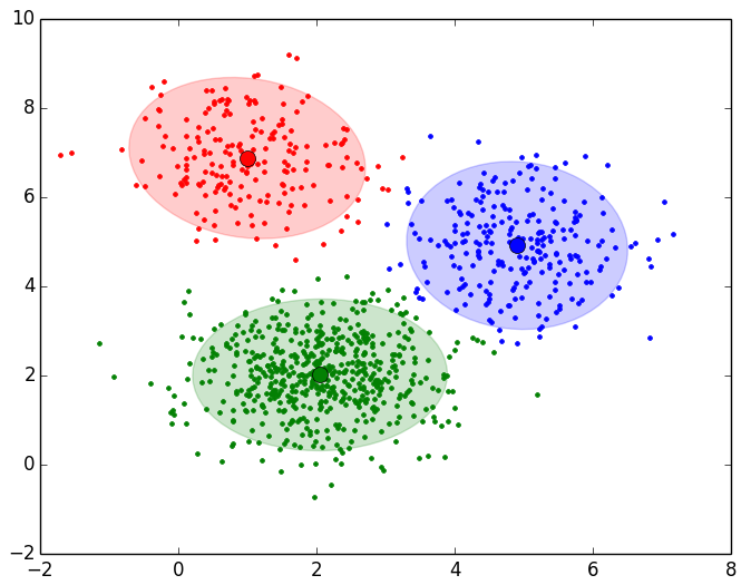
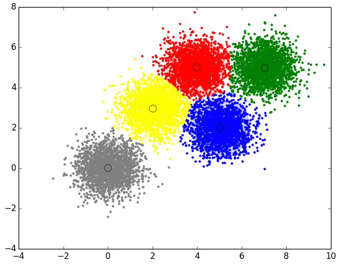
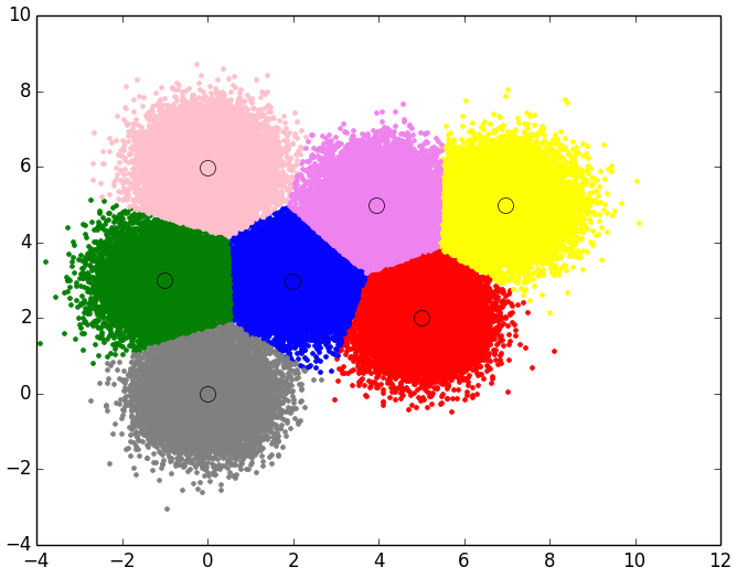
For the rest of the data sets we have the following results, plotted in 2 dimensions:
- Final EM result for Data Set 2 with 999 points and 3 Clusters:
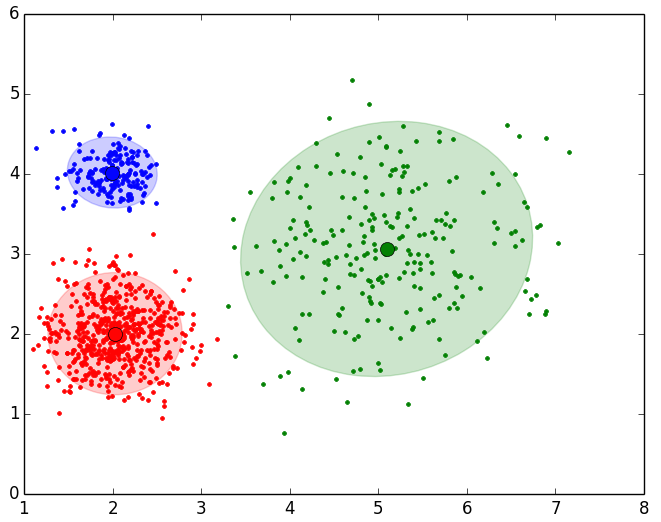
- Final EM result for Data Set 3 with 10000 points and 5 Clusters
- Final EM result for Data Set 4 with 100000 points and 7 Clusters
Expectation-maximization (Gaussian mixture models) with scikit-learn
The “scikit-learn” library implements Gaussian mixture models (GMM), which is EM assuming normal (or Gaussian) probability distributions; that is, the data to be Clustered is assumed to have been generated by Gaussian distributions, hence the name “Gaussian mixture models”. This GMM implementation is quite optimized, and it can be run in different ways depending on the parameters you pass to it.
Since libraries in general, and this Machine Learning one in particular, evolve and change over time, we’re not going to explain every parameter that can be passed to the constructor of the sklearn.cluster.GMM() class (that’s what the scikit-learn documentation is for), but we will show the parameters that are considered important for any EM implementation (or in this case, GMM).
In version 0.17 of the library (the latest stable version at the time of writing this book) the constructor of the GMM class has the following parameters (if you don’t specify them, they take default values):
class sklearn.mixture.GMM(n_components=1, covariance_type='diag', random_state=None, thresh=None,tol=0.001, min_covar=0.001, n_iter=100, n_init=1, params='wmc', init_params='wmc', verbose=0)
For GMM to run correctly with the data set you use, you must properly define the following two required and important parameters:
- n_components: The number of normal distributions (or Clusters) we want to obtain to group the objects in the data set.
- n_iter: The maximum number of runs of the expectation and maximization steps, in case the means of the normal distributions don’t converge.
Optionally, we can define a series of parameters with the values we see fit, the most practical ones (in the author’s opinion) being the following:
- tol: With this value we set the threshold, tolerance or margin of error for convergence.
- params: We tell it which parameters it should update in the maximization step.
Once the GMM object is built, we must call the appropriate methods so it calculates the parameters mentioned above. In this case, and for the example we show below, we call the fit(x) method, passing it a list of points (each point in a numpy array); it gives us back the probability ‘π’ of belonging to the normal distributions (in the weights_ attribute) and the mean of the normal distributions (in the means_ attribute). Then, by calling the predict(x) method, passing it a list with the points of the data set, it calculates a list aligned with the list of points we passed, telling us which normal distribution or Cluster each point belongs to.
Below is the complete script, showing the GMM results for one of the 4 data sets:
# -*- coding: utf-8 -*-
__author__ = 'RicardoMoya'

import numpy as np
import matplotlib.pyplot as plt
from matplotlib.patches import Ellipse
from sklearn.mixture import GMM

# Constant
DATASET1 = "./dataSet/DS_3Clusters_999Points.txt"
DATASET2 = "./dataSet/DS2_3Clusters_999Points.txt"
DATASET3 = "./dataSet/DS_5Clusters_10000Points.txt"
DATASET4 = "./dataSet/DS_7Clusters_100000Points.txt"
NUM_CLUSTERS = 3
MAX_ITERATIONS = 10
CONVERGENCE_TOLERANCE = 0.001
COLORS = ['red', 'blue', 'green', 'yellow', 'gray', 'pink', 'violet', 'brown',
          'cyan', 'magenta']


def dataset_to_list_points(dir_dataset):
    """
    Read a txt file with a set of points and return a list of objects Point
    :param dir_dataset:
    """
    points = list()
    with open(dir_dataset, 'rt') as reader:
        for point in reader:
            points.append(np.asarray(map(float, point.split("::"))))
    return points


def print_results(means_clusters, probability_clusters, label_cluster_points):
    print '\n\nFINAL RESULT:'
    for i, c in enumerate(means_clusters):
        print '\tCluster %d' % (i + 1)
        print '\t\tNumber Points in Cluster %d' % label_cluster_points.count(i)
        print '\t\tCentroid: %s' % str(means_clusters[i])
        print '\t\tProbability: %02f%%' % (probability_clusters[i] * 100)


def plot_ellipse(center, covariance, alpha, color):

    # eigenvalues and eigenvector of matrix covariance
    eigenvalues, eigenvector = np.linalg.eigh(covariance)
    order = eigenvalues.argsort()[::-1]
    eigenvector = eigenvector[:, order]

    # Calculate Angle of ellipse
    angle = np.degrees(np.arctan2(*eigenvector[:, 0][::-1]))

    # Calculate with, height
    width, height = 4 * np.sqrt(eigenvalues[order])

    # Ellipse Object
    ellipse = Ellipse(xy=center, width=width, height=height, angle=angle,
                      alpha=alpha, color=color)

    ax = plt.gca()
    ax.add_artist(ellipse)

    return ellipse


def plot_results(points, means_clusters, label_cluster_points,
                 covars_matrix_clusters):
    plt.plot()
    for nc in range(len(means_clusters)):
        # Plot points in cluster
        points_cluster = list()
        for i, p in enumerate(label_cluster_points):
            if p == nc:
                plt.plot(points[i][0], points[i][1], linestyle='None',
                         color=COLORS[nc], marker='.')
                points_cluster.append(points[i])
        # Plot mean
        mean = means_clusters[nc]
        plt.plot(mean[0], mean[1], 'o', markerfacecolor=COLORS[nc],
                 markeredgecolor='k', markersize=10)

        # Plot Ellipse
        plot_ellipse(mean, covars_matrix_clusters[nc], 0.2, COLORS[nc])

    plt.show()


def expectation_maximization(dataset, num_clusters, tolerance, max_iterations):
    # Read data set
    points = dataset_to_list_points(dataset)

    # Object GMM
    gmm = GMM(n_components=num_clusters, covariance_type='full', tol=tolerance,
              n_init=max_iterations, params='wmc')

    # Estimate Model (params='wmc'). Calculate, w=weights, m=mean, c=covars
    gmm.fit(points)

    # Predict Cluster of each point
    label_cluster_points = gmm.predict(points)

    means_clusters = gmm.means_
    probability_clusters = gmm.weights_
    covars_matrix_clusters = gmm.covars_


    # Print final result
    print_results(means_clusters, probability_clusters,
                  label_cluster_points.tolist())

    # Plot Final results
    plot_results(points, means_clusters, label_cluster_points,
                 covars_matrix_clusters)


if __name__ == '__main__':
    expectation_maximization(DATASET1, NUM_CLUSTERS, CONVERGENCE_TOLERANCE,
                             MAX_ITERATIONS)
Next we explain in detail how we built the script. All the work happens in the expectation_maximization(dataset, num_clusters, tolerance, max_iterations) method, which receives as parameters the data set, the number of Clusters, the convergence threshold and the maximum number of iterations. We call this method from ‘main’, and the parameters passed to it are constants defined at the beginning of the script:
# Constant
DATASET1 = "./dataSet/DS_3Clusters_999Points.txt"
DATASET2 = "./dataSet/DS2_3Clusters_999Points.txt"
DATASET3 = "./dataSet/DS_5Clusters_10000Points.txt"
DATASET4 = "./dataSet/DS_7Clusters_100000Points.txt"
NUM_CLUSTERS = 3
MAX_ITERATIONS = 10
CONVERGENCE_TOLERANCE = 0.001
COLORS = ['red', 'blue', 'green', 'yellow', 'gray', 'pink', 'violet', 'brown',
          'cyan', 'magenta']

----------------------------------------------------------------------------------

if __name__ == '__main__':
    expectation_maximization(DATASET1, NUM_CLUSTERS, CONVERGENCE_TOLERANCE, MAX_ITERATIONS)
Inside the expectation_maximization() method we start by reading the data (points) from the data set we indicate, putting those points into a list of numpy arrays:
def expectation_maximization(dataset, num_clusters, tolerance, max_iterations):
    # Read data set
    points = dataset_to_list_points(dataset)
We initialize the GMM class object (from scikit-learn), passing it as parameters the number of Clusters (n_components), the tolerance threshold (tol), the maximum number of iterations (n_init) and the parameters to update in the maximization step (params):
gmm = GMM(n_components=num_clusters, covariance_type='full', tol=tolerance, n_init=max_iterations, params='wmc')
We call the fit(x) method and the predict(x) method, passing them the list of points (numpy array), so they calculate the parameters of the distributions and the Cluster each point belongs to:
# Estimate Model (params='wmc'). Calculate, w=weights, m=mean, c=covars
gmm.fit(points)

# Predict Cluster of each point
label_cluster_points = gmm.predict(points)
We get the values of the mean of the Cluster distributions (means_clusters), the probability of belonging to each Cluster (probability_clusters) and the covariance matrix (covars_matrix_clusters), which we’ll use to draw an area of influence for the Cluster:
means_clusters = gmm.means_
probability_clusters = gmm.weights_
covars_matrix_clusters = gmm.covars_
Finally we implement two methods: one to print the results (midpoint, number of points in each Cluster and the membership probability) and another to plot (with the matplotlib library) the midpoints and the points assigned to each Cluster:
print_results(means_clusters, probability_clusters, label_cluster_points.tolist())
plot_results(points, means_clusters, label_cluster_points, covars_matrix_clusters)
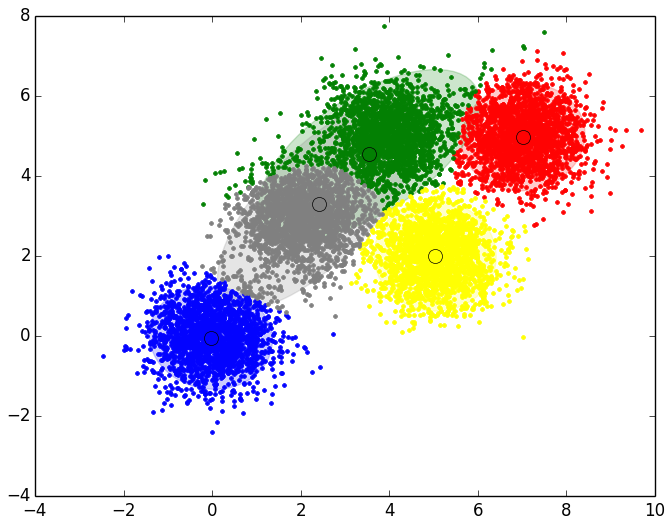
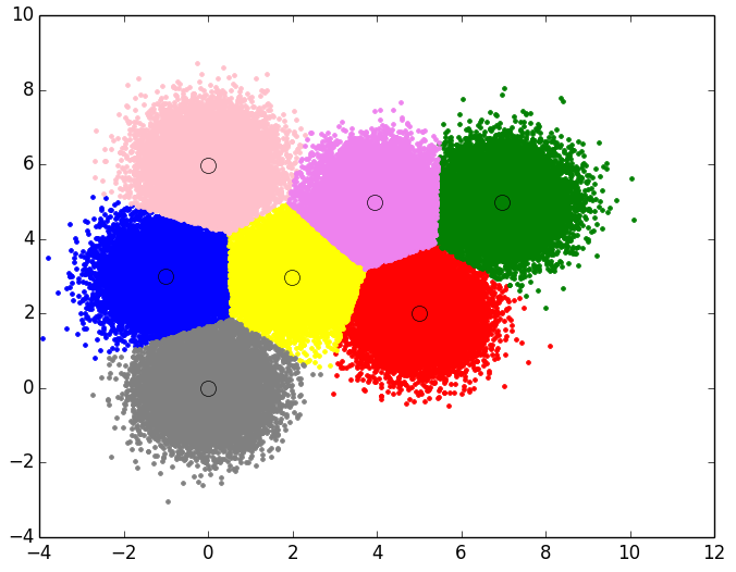
Applying this script to the 4 proposed data sets, we get the following results:
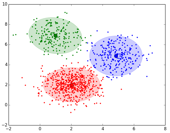
- Data Set 1: 3 Clusters and 999 points:
FINAL RESULT:
	Cluster 1
		Number Points in Cluster 552
		Centroid: [ 2.03233538  2.00853155]
		Probability: 55.061812%
	Cluster 2
		Number Points in Cluster 253
		Centroid: [ 4.85698668  4.87166594]
		Probability: 25.632025%
	Cluster 3
		Number Points in Cluster 194
		Centroid: [ 0.98302746  6.88925282]
		Probability: 19.306162%
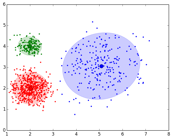
- Data Set 2: 3 Clusters and 999 points:
FINAL RESULT:
	Cluster 1
		Number Points in Cluster 186
		Centroid: [ 1.99735203  4.01744321]
		Probability: 18.639301%
	Cluster 2
		Number Points in Cluster 242
		Centroid: [ 5.08393907  3.06038361]
		Probability: 24.320184%
	Cluster 3
		Number Points in Cluster 571
		Centroid: [ 2.02688227  2.00363213]
		Probability: 57.040515%
- Data Set 3: 5 Clusters and 10000 points:
FINAL RESULT:
	Cluster 1
		Number Points in Cluster 1971
		Centroid: [ 7.02380409  4.97477739]
		Probability: 19.503728%
	Cluster 2
		Number Points in Cluster 1935
		Centroid: [-0.03006596 -0.03848878]
		Probability: 18.591360%
	Cluster 3
		Number Points in Cluster 2074
		Centroid: [ 3.5474937   4.55700106]
		Probability: 19.963076%
	Cluster 4
		Number Points in Cluster 2012
		Centroid: [ 5.0348546   2.00442168]
		Probability: 19.923560%
	Cluster 5
		Number Points in Cluster 2008
		Centroid: [ 2.41381883  3.29885127]
		Probability: 22.018275%
- Data Set 4: 7 Clusters and 100000 points:
FINAL RESULT:
	Cluster 1
		Number Points in Cluster 14270
		Centroid: [ 5.00790293  2.00510173]
		Probability: 14.267490%
	Cluster 2
		Number Points in Cluster 14219
		Centroid: [-0.99805653  2.99389472]
		Probability: 14.217667%
	Cluster 3
		Number Points in Cluster 14407
		Centroid: [ 6.97099609  4.99667353]
		Probability: 14.545643%
	Cluster 4
		Number Points in Cluster 14090
		Centroid: [ 1.99643225  2.98306353]
		Probability: 13.934259%
	Cluster 5
		Number Points in Cluster 14329
		Centroid: [ 0.0083095  -0.00197396]
		Probability: 14.331673%
	Cluster 6
		Number Points in Cluster 14366
		Centroid: [ -4.37927760e-03   5.98768206e+00]
		Probability: 14.355278%
	Cluster 7
		Number Points in Cluster 14319
		Centroid: [ 3.940767    4.97634401]
		Probability: 14.347991%
“Expectation-Maximization in Python and Scikit-learn, with Examples” by Ricardo Moya at jarroba.com, licensed under Creative Commons Attribution-NonCommercial-ShareAlike 3.0. Registered at Safe Creative.

You may also like
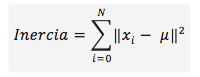
K-means in Python and Scikit-learn, with Examples
K-means is a clustering method that splits objects into K groups by minimizing inertia. Learn how it works and how to use it in Python with scikit-learn.
Selecting the Optimal Number of Clusters
One of the problems when applying a Clustering method (K-means or EM) is choosing the number of Clusters. Learn the elbow method, dendrograms and the gap.
Leave a comment