
What is a model (and why a straight line already counts as one)
What a model is, what training and predicting mean, with a line you fit by dragging points. And why a model does not understand its data. AI course, 0.4.

AI from the First Bit › Level 0 — How a machine sees the world part 4 of 4
“Model”, “train” and “predict” are words that come up constantly when talking about AI, and all three fit in a straight line: the model is the line, training is placing it among the points, and predicting is reading its height at a new point.
Try this first
Open the Regression & MLE tool. You will see ten points and a line that passes between them. The vertical gray lines joining each point to the line are the residuals: how far off the line is at that point. On the right, MSE (loss) is 0.236. MSE is the mean squared error, and loss is the name given to the error you want to make small: each error is squared, the ten are added up and the total is divided by ten. (Further down you have the calculation worked out point by point, in case you want to repeat it on paper.)
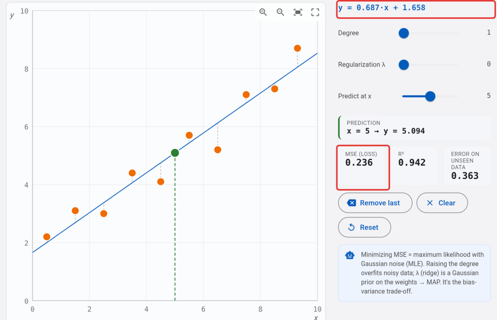
Take the fifth point from the left and drag it upward. The line tilts a little toward it and the MSE goes up: the farther you move it, the more. You have not touched the line: it has recalculated itself so that the total error is the smallest possible with the new points. Look also at the equation at the top right, y = 0.687·x + 1.658: while you drag, those two numbers change.
Now click Clear and click in five places on the chart to place your own points. With each click, the line repositions itself. Pay attention to the first three. With one point, the MSE is 0, but infinitely many lines pass through one point and all of them get it right; the tool picks the horizontal one. With two, the line passes exactly through both and the MSE is still 0. From the third on, if they are not aligned, no line passes through all of them and the MSE stops being 0. A line has two numbers to adjust: with two points it always gets it right, even though it has not learned anything.
With three or four points, a red overfitting warning may appear. The tool runs a test: it removes one point, fits the line with the others and checks how much it misses the one it removed, and it repeats this with every point. With so few, the line clings to the ones it has and misses a lot on the one it has not seen. What makes the warning go away is adding more points: with five it usually disappears. Overfitting is covered in detail later, in Fitting a curve.
What just happened
You have just done all three things.
The data are the points. Each one is a pair of numbers: where it is horizontally (x) and vertically (y). They could be hours of study and an exam grade, square meters and the price of an apartment, or anything that is measured in two numbers.
The model is the line. A line is fixed by just two numbers: how much it tilts and at what height it crosses the vertical axis. The tool writes it at the top right; with the ten starting points it is y = 0.687·x + 1.658. Those two numbers (0.687 and 1.658) are the model: everything it has learned from the ten points fits in there.
Training is searching for those two numbers. Not just any line will do: you look for the one that makes the mean of the squared errors as small as possible, the MSE you see on screen. They are squared so that an error above and another below do not cancel each other out, and so that a large error weighs much more than a small one. That is why the method is called least squares, and it is not new: Adrien-Marie Legendre published it in 1805, and in 1809 Carl Friedrich Gauss claimed that he had been using it since 1795 (Least squares, on Wikipedia).
Tip
To do it by hand (you can skip this box; the rest of the article does not need it)
With the tool’s ten starting points, the line and its error come out in three steps. Σ means “the sum over all the rows”, x̄ is the mean of the x values and ȳ the mean of the y values.
1. The means. Add up the ten x values and divide by 10: x̄ = 4.98. Same with the y values: ȳ = 5.08.
2. The slope (b) and the intercept (a). The least-squares formulas for a line are:
b = Σ (x − x̄)·(y − ȳ) / Σ (x − x̄)² and a = ȳ − b·x̄
(They come from looking for the line with the smallest sum of squared errors; you do not need to derive them to use them.) The table works it out point by point:
| x | y | x − x̄ | y − ȳ | (x − x̄)·(y − ȳ) | (x − x̄)² |
|---|---|---|---|---|---|
| 0.5 | 2.2 | −4.48 | −2.88 | 12.9024 | 20.0704 |
| 1.5 | 3.1 | −3.48 | −1.98 | 6.8904 | 12.1104 |
| 2.5 | 3.0 | −2.48 | −2.08 | 5.1584 | 6.1504 |
| 3.5 | 4.4 | −1.48 | −0.68 | 1.0064 | 2.1904 |
| 4.5 | 4.1 | −0.48 | −0.98 | 0.4704 | 0.2304 |
| 5.5 | 5.7 | 0.52 | 0.62 | 0.3224 | 0.2704 |
| 6.5 | 5.2 | 1.52 | 0.12 | 0.1824 | 2.3104 |
| 7.5 | 7.1 | 2.52 | 2.02 | 5.0904 | 6.3504 |
| 8.5 | 7.3 | 3.52 | 2.22 | 7.8144 | 12.3904 |
| 9.3 | 8.7 | 4.32 | 3.62 | 15.6384 | 18.6624 |
| Sum | 55.4760 | 80.7360 |
b = 55.476 / 80.736 = 0.68713 and a = 5.08 − 0.68713 × 4.98 = 1.6581. The tool writes them rounded: y = 0.687·x + 1.658.
3. The error at each point and the MSE. For each point, the prediction is a + b·x; the error is what lies between the point and the line (y − prediction); and it is squared:
| x | y | prediction a + b·x | error = y − prediction | error² |
|---|---|---|---|---|
| 0.5 | 2.2 | 2.002 | 0.198 | 0.0393 |
| 1.5 | 3.1 | 2.689 | 0.411 | 0.1691 |
| 2.5 | 3.0 | 3.376 | −0.376 | 0.1413 |
| 3.5 | 4.4 | 4.063 | 0.337 | 0.1135 |
| 4.5 | 4.1 | 4.750 | −0.650 | 0.4227 |
| 5.5 | 5.7 | 5.437 | 0.263 | 0.0690 |
| 6.5 | 5.2 | 6.124 | −0.924 | 0.8546 |
| 7.5 | 7.1 | 6.812 | 0.288 | 0.0832 |
| 8.5 | 7.3 | 7.499 | −0.199 | 0.0395 |
| 9.3 | 8.7 | 8.048 | 0.652 | 0.4246 |
| Sum | 2.3569 |
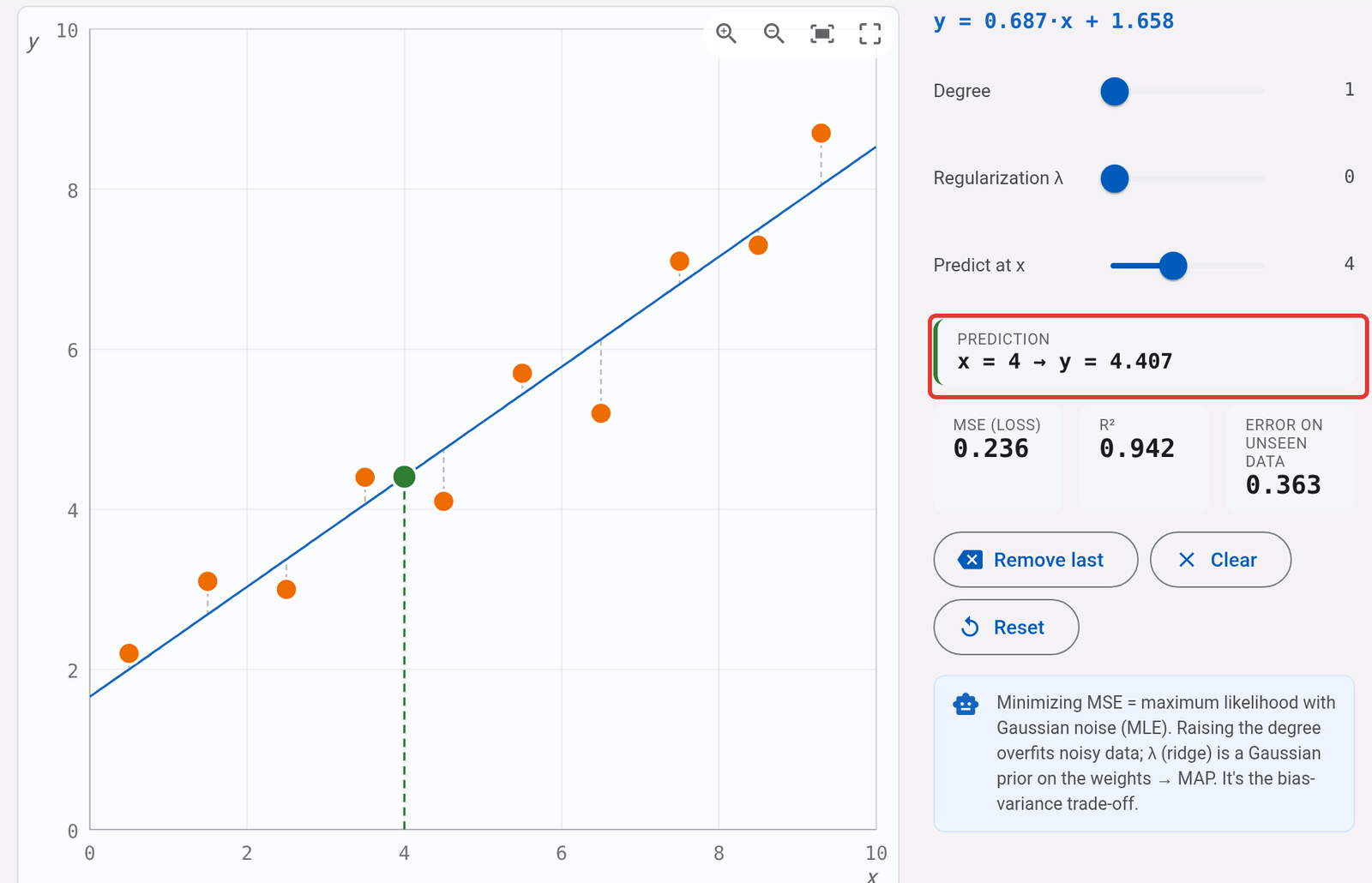
The mean of those ten squared errors is 2.3569 / 10 = 0.236: the MSE the tool shows. (Depending on how many decimal places you round to along the way, your result may be off by a thousandth.) With the same line, the prediction at x = 4 is 1.6581 + 0.68713 × 4 = 4.407.
For a line, those two numbers can be calculated in one go with a formula, and that is what the tool does every time you move a point. Large models have so many numbers that no formula gets them all at once, and they are adjusted in small steps, correcting a little on each pass (that way of training is the one in How a machine learns). The underlying idea is the same: look for the numbers that make the error smallest.
Predicting is using the line with an x that was not in the data. Open the same tool with the prediction at x = 4: the green point on the line and the reading x = 4 → y = 4.407. There is nothing more behind it: a prediction is the height of the line at that point.
The name of all this, regression, also has a history. It comes from a study by Francis Galton in 1886 about heights. Galton compared each child’s height with the mean of their two parents’ heights, and saw that the children strayed from the population’s average height less than their parents did: if the mean of the two parents was, for example, 6 cm above the average, the children also tended to be above it, but only about 4 cm: closer to the average. The same happened below the average with short parents. He calculated that the children stayed at around two thirds of their parents’ distance from the mean: they “regressed” toward it (Regression toward the mean, on Wikipedia). The name stuck for the method even though it has nothing to do with going backward.
The classic mistake
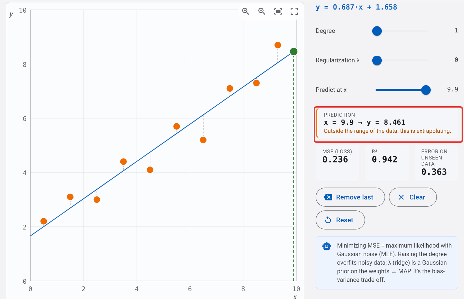
You might think a model understands the data. The one in this article is a line: it does not know what the points are, only where they are. If the points were hours of study and grades, the line would keep rising without limit, and with 50 hours it would “predict” a grade of 36 out of 10. It is not a calculation error: the line does exactly what it was asked; what it does not know is when it has stopped making sense. The tool does point it out to you: ask for a prediction at x = 9.9, beyond the last point, and the warning “Outside the range of the data: this is extrapolating.” appears below it. That warning does not come from the line: whoever made the tool put it there. In large models the same thing happens, with many more numbers.
What changes in your work
When an AI tool gives you a figure or a recommendation, it is doing the same thing as the line: applying what it learned from examples. It does not know whether your case looks like those examples. If you ask about something very different from the usual (an atypical customer, a new product, an odd year), the answer comes out with the same confidence, even though it no longer means anything. Before trusting the answer, ask yourself whether your case resembles what it learned from.
Try it yourself
In Regression & MLE, click Reset to go back to the ten starting points. Raise the first point on the left a little and see how much the tilt of the line changes. Put it back with Reset and do the same with the fifth, which is toward the middle. Which one moves the line more? Why do you think a point at one end weighs more than one in the middle?
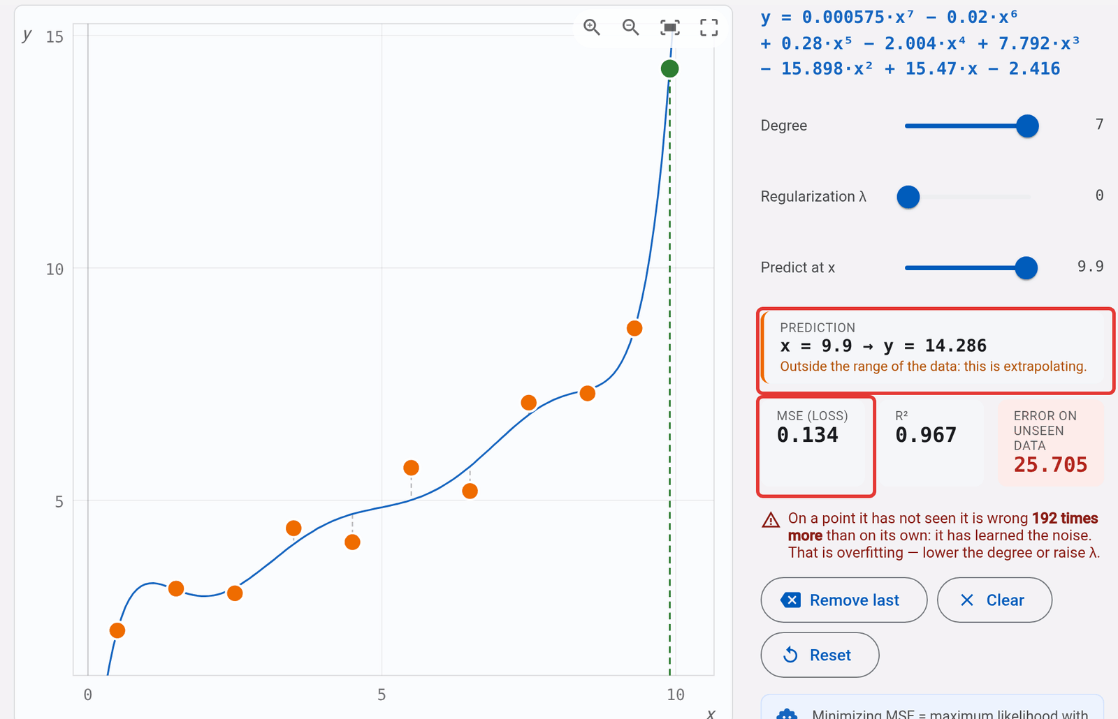
And for the next step in the series: open the same tool with degree 7. It is no longer a line: the curve twists to get closer to the points, the MSE drops (from 0.236 to 0.134) and at the edges it shoots off. Now ask for the same prediction at x = 9.9 with this curve: the line said 8.461; the curve says 14.286. Is it a better model? Keep the answer for later (it is the subject of Fitting a curve).
Further reading
- At Jarroba, by Ricardo Moya: What Is Machine Learning?, with the concepts of training set, model and overfitting explained with charts; and the Map: Learning Algorithms and Concepts of (Deep) Machine Learning, to see where regression fits in with everything else.
- Least squares, on Wikipedia: the full history of the method, including the dispute between Legendre and Gauss.
“What is a model (and why a straight line already counts as one)” by Ramón Invarato at jarroba.com, licensed under Creative Commons Attribution-NonCommercial-ShareAlike 3.0. Registered at Safe Creative.

You may also like

A corrupted bit: how to fix it without knowing which one it is
How a computer finds and fixes a corrupted bit without knowing which one it is: the Hamming code, its limits and SECDED. AI course, 0.3.

An image is a table of numbers
A photo is a table of numbers: three per pixel, red, green and blue. See it on an apple and why its red is thousands of numbers. AI course, 0.2.
Leave a comment